Working with OSM data at the command line
OpenStreetMap is a community-driven initiative to create and provide free geographic data, such as street maps, to anyone. At the time of this post, 6.9 million registered users have contributed 6.4B nodes, 700M ways, and 8.2M relations. The project provides a wealth of free global geospatial data, if you know how to use it.
Getting set up
There are many tools you can use to interact with OSM data. The goal here is not to cover all of them, but rather to focus on a few that I have worked with recently.
I use a Mac and this post assumes you are using one, too.
Install
You can run the following commands in the terminal to install a few utilities you will need to follow along with this walkthrough.
/bin/bash -c "$(curl -fsSL https://raw.githubusercontent.com/Homebrew/install/master/install.sh)"brew install osmium-toolThis command takes a little while to complete, so now is a great time to grab a beer.
brew install gdalProject directory
To keep things organized on your machine, let’s work out of a new project directory. Run the following commands in your terminal.
mkdir osm-at-the-cmd-line
cd osm-at-the-cmd-line
Download
You can download OSM data in a variety of ways, but I have found it easiest to download from Geofabrik's free download server, as they have region and subregion extracts readily available for download.
For this walkthrough, let’s download the latest extract of Belgium. Run the following command in your terminal.
curl -O https://download.geofabrik.de/europe/belgium-latest.osm.pbfIf you don’t want to use curl, you can download the latest extract directly by clicking this link. Be sure to move the downloaded file into the root of our osm-at-the-cmd-line directory.
Working with the data
With the latest extract of Belgium in our new project directory, we can get started looking at the data.
Filtering by bounding box
When working on a laptop or other local machine, it is likely we run into some limit on processing power. While the Belgium dataset is relatively small, this is a great opportunity to get started with one of the tools we installed earlier, osmium-tool. Let’s extract a small portion of the larger dataset using a bounding box.
I used a website recommended in the OSM wiki to create a rough bounding box around Brussels, the capital of Belgium. You’ll want to click each of the corners to drag them until the bounding box envelops Brussels, then switch Copy & Paste to CSV to get coordinates in the correct format (minimum latitude, minimum longitude, maximum latitude, maximum longitude). I ended up with 4.134979,50.671224,4.658203,50.972265, but your mileage may vary.
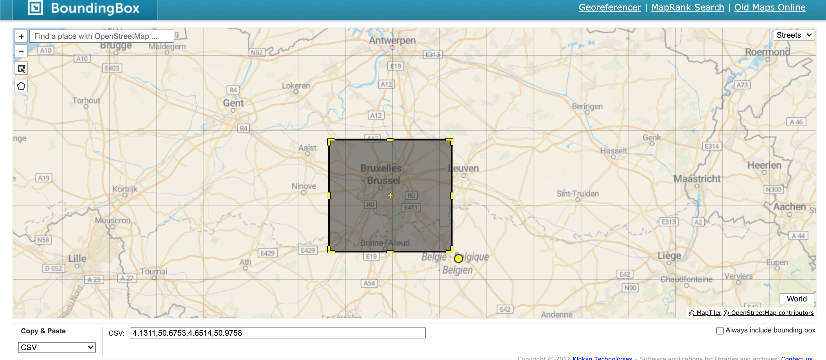
We can pass this bounding box to the osmium extract command using the --bbox option. This selects only the features in the larger file that intersect with this area. The -o option tells osmium where to output the data, in this case brussels.osm.pbf.
osmium extract --bbox 4.134979,50.671224,4.658203,50.972265 belgium-latest.osm.pbf -o brussels.osm.pbfbrussels.osm.pbf should now contain only nodes, ways, and relations in the given bounding box.
Filtering by tags
Every element in OSM can be labelled with tags to describe features such as class, use case, or even attributes like a roadway’s speed limit. For this walkthrough, we can use a tag called highway to extract the most important roadways in Brussels. Three of the most important roadways in OSM are tagged as motorway, trunk, and primary.
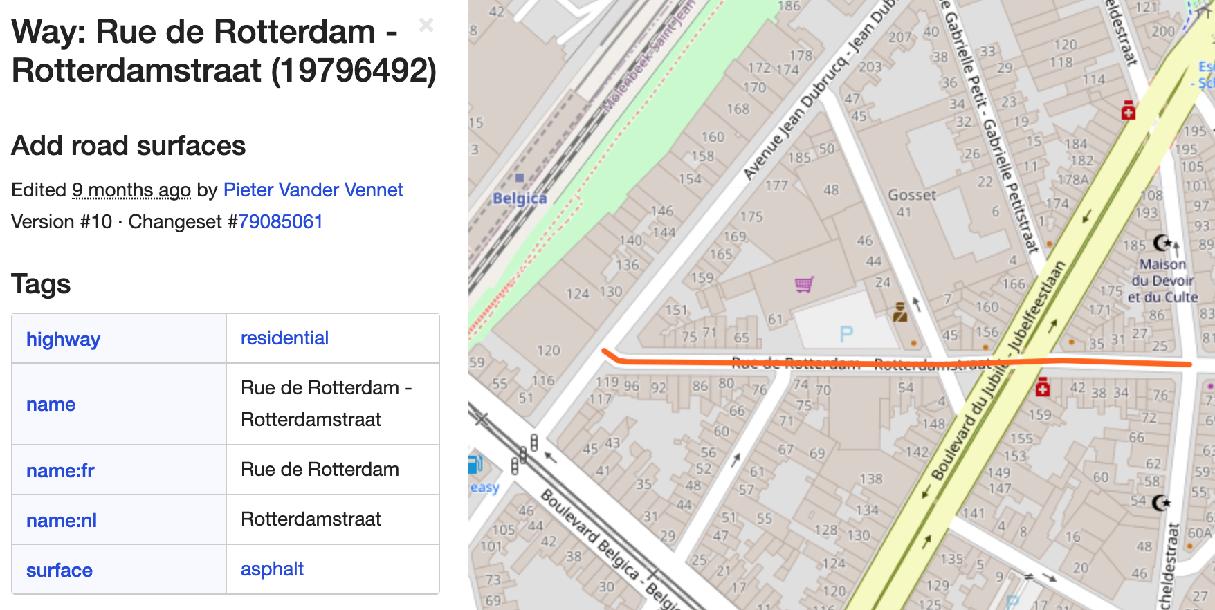
To do this, we can use the osmium tags-filter command.
osmium tags-filter -o ways.osm.pbf brussels.osm.pbf w/highway=motorway,trunk,primaryAfter running the above command, the ways.osm.pbf file now contains only ways within the Brussels bbox with the highway tags of motorway, trunk, primary.
Visualizing the data
Now that we have the major roadways in Brussels, it’s time to visualize the data. I’ve found one of the quickest ways to visualize geospatial data without any initial set up is kepler.gl. The one catch is Kepler requires the data to be formatted as CSV, JSON, GeoJSON or a saved map JSON.
A quick way to transform your PBF data is to GeoJSON is using GDAL’s ogr2ogr, which we installed earlier in the walkthrough.
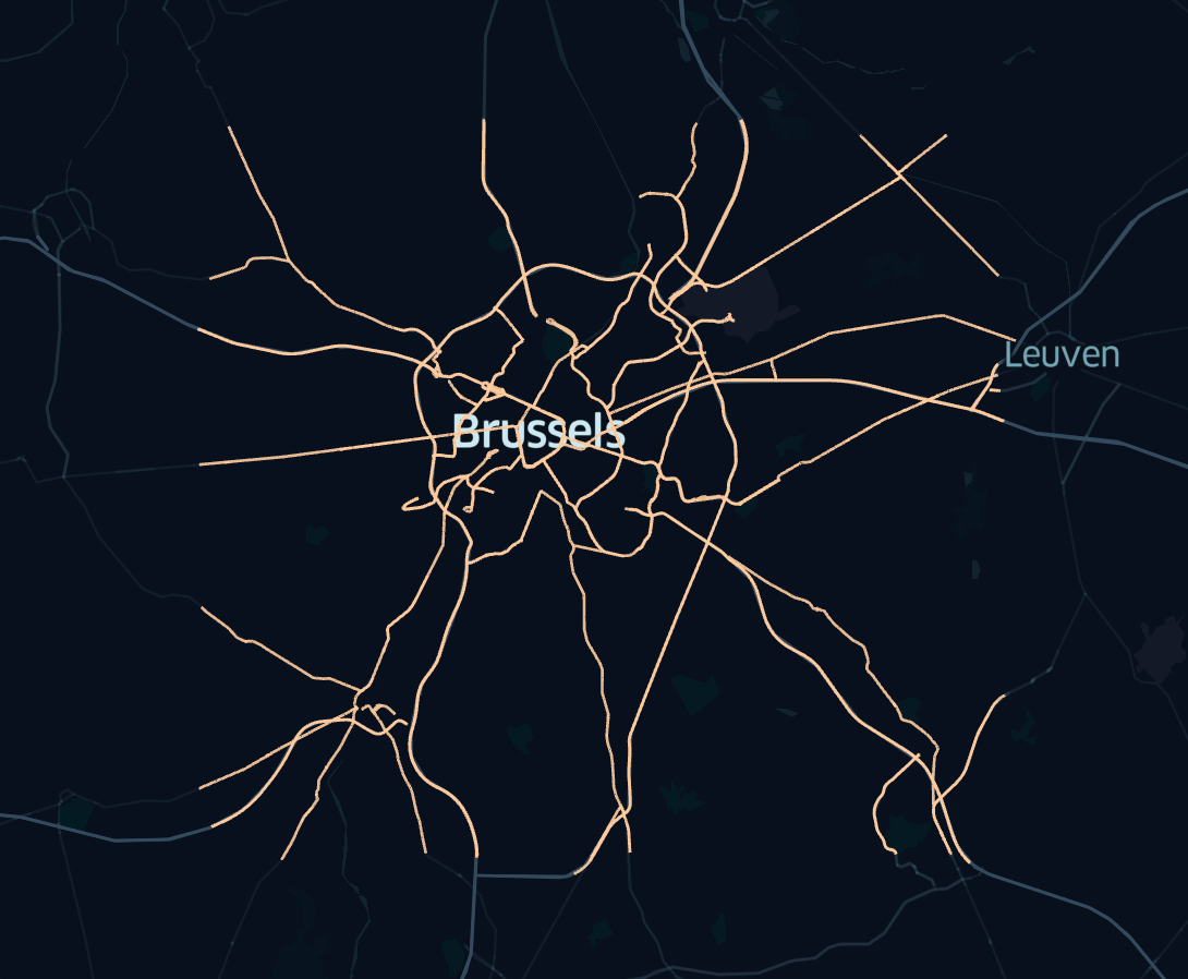
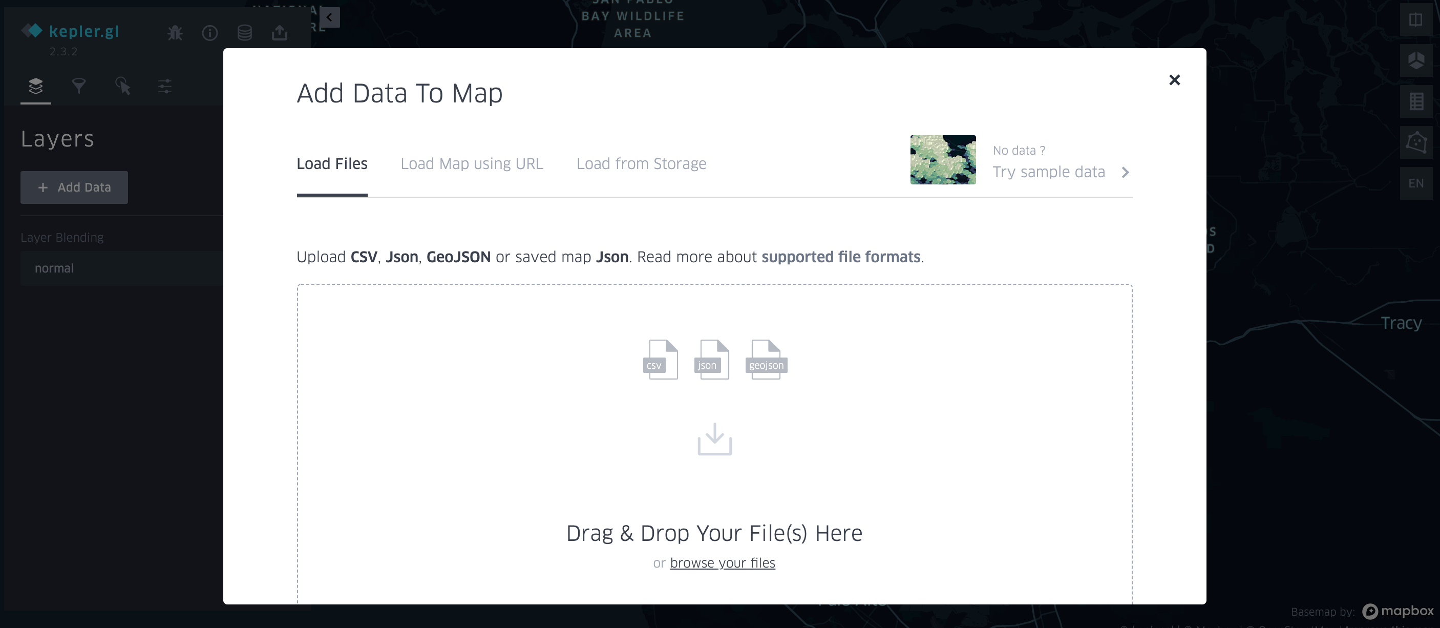
ogr2ogr -f GeoJSON output_lines.geojson ways.osm.pbf linesOpen kepler.gl and upload your output_lines.geojson file.
Once the data has loaded, you should see something like this: